
Algo#4 Coping with Hardness
Backtracking
The General Backtracking Method
\begin{algorithm}
\caption{BACKTRACKREC}
\begin{algorithmic}
\Input  Explicit or implicit description of the sets $X_1,X_2,\dots,X_n$.
\Output A solution vector $v = (x_1,x_2,\dots,x_i),0 \leq i \leq n$.
\State $v \gets ()$
\State $flag \gets$ \False
\State \Call{advance}{1}
\If{$flag$}
\State output $v$
\Else
\State output "no solution"
\EndIf
\Procedure{advance}{$k$}
\For{each $x \in X_k$}
\State $x_k \gets x$; append $x_k$ to $v$
\If{$v$ is a final solution}
\State set $flag \gets$ \True and exit
\Elif{$v$ is partial}
\State \Call{advance}{$k+1$}
\EndIf
\EndFor
\EndProcedure
\end{algorithmic}
\end{algorithm}
\begin{algorithm}
\caption{BACKTRACKINER}
\begin{algorithmic}
\Input  Explicit or implicit description of the sets $X_1,X_2,\dots,X_n$.
\Output A solution vector $v = (x_1,x_2,\dots,x_i),0 \leq i \leq n$.
\State $v \gets ()$
\State $flag \gets$ \False
\State $k \gets 1$
\While{$k \geq 1$}
\While{$X_k$ is not exhausted}
\State $x_k \gets$ next element in $X_K$; append $x_k$ to $v$
\If{$v$ is a final solution}
\State set $flag \gets$ \True and exit from the two while loops.
\Elif{$v$ is partial}
\State $k \gets k + 1$ \Comment{advance}
\EndIf
\EndWhile
\State Reset $X_k$ so that the next element is the first.
\State $k \gets k-1$ \Comment{backtrack}
\EndWhile
\If{$flag$}
\State output $v$
\Else
\State output "no solution"
\EndIf
\end{algorithmic}
\end{algorithm}
The 3-Coloring Problem
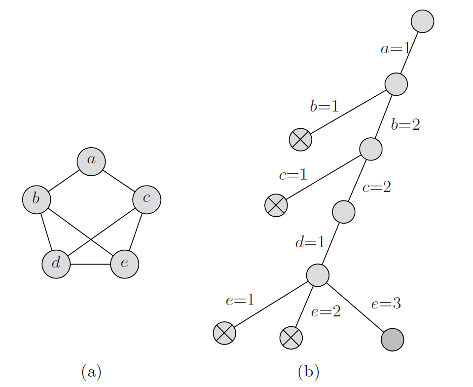
Consider the problem 3-coloring: Given an undirected graph , it is required to color each vertex in with one of three colors, say , , and , such that no two adjacent vertices have the same color. We call such a coloring legal; otherwise, if two adjacent vertices have the same color, it is illegal. A coloring can be represented by an -tuple such that , .
\begin{algorithm}
\caption{3-COLORREC}
\begin{algorithmic}
\Input An undirected graph $G = (V,E)$.
\Output A $3$-coloring $c[1..n]$ of the vertices of $G$, where each $c[j]$ is $1$, $2$, and $3$.
\For{$k \gets 1$ \To $n$}
\State $c[k] \gets 0$
\EndFor
\State $flag \gets$ \False
\State \Call{graphcolor}{1}
\If{$flag$}
\State output $c$
\Else
\State output "no solution"
\EndIf
\Procedure{graphcolor}{$k$}
\For{$color = 1$ \To $3$}
\State $c[k] \gets color$
\If{$c$ is a legal coloring}
\State set $flag \gets$ \True and exit
\Elif{$c$ is partial}
\State \Call{graphcolor}{$k+1$}
\EndIf
\EndFor
\EndProcedure
\end{algorithmic}
\end{algorithm}
\begin{algorithm}
\caption{3-COLORITER}
\begin{algorithmic}
\Input An undirected graph $G = (V,E)$.
\Output A $3$-coloring $c[1..n]$ of the vertices of $G$, where each $c[j]$ is $1$, $2$, or $3$.
\For{$k \gets 1$ \To $n$}
\State $c[k] \gets 0$
\EndFor
\State $flag \gets$ \False
\State $k \gets 1$
\While{$k \ge 1$}
    \While{$c[k] \le 2$}
        \State $c[k] \gets c[k] + 1$
        \If{$c$ is a legal coloring}
            \State set $flag \gets$ \True and exit from the two while loops.
        \ElsIf{$c$ is partial}
            \State $k \gets k + 1$ \Comment{advance}
        \EndIf
    \EndWhile
    \State $c[k] \gets 0$
    \State $k \gets k - 1$ \Comment{backtrack}
\EndWhile
\If{$flag$}
\State output $c$
\Else
\State output "no solution"
\EndIf
\end{algorithmic}
\end{algorithm}
Below is the implementation of these pseudocodes in Python(Adjacency list):
1 | G = { |
The 8-Queens Problem
The classical 8-queens can be stated as follows. How can we arrange eight queens on an chessboard so that no two queens can attack each other? Two queens can attack each other if they are in the same row, column, or diagonal.
Consider a chessboard of size . Since no two queens can be put in the same row, each queen is in a different row. Since there are four positions in each row, there are possible configurations. Each possible configuration can be described by a vector with four components .
\begin{algorithm}
\caption{4-QUEENSITER}
\begin{algorithmic}
\Input None.
\Output Vector $x[1..4]$ corresponding to the solution of the $4$-queens problem.
\For{$k \gets 1$ \To $4$}
\State $x[k] \gets 0$ \Comment{no queens are placed on the chessboard}
\EndFor
\State $flag \gets$ \False
\State $k \gets 1$
\While{$k \ge 1$}
    \While{$x[k] \le 3$}
        \State $x[k] \gets x[k] + 1$
        \If{$x$ is a legal placement}
            \State set $flag \gets$ \True and exit from the two while loops.
        \ElsIf{$x$ is partial}
            \State $k \gets k + 1$ \Comment{advance}
        \EndIf
    \EndWhile
    \State $x[k] \gets 0$
    \State $k \gets k - 1$ \Comment{backtrack}
\EndWhile
\If{$flag$}
\State output $x$
\Else
\State output "no solution"
\EndIf
\end{algorithmic}
\end{algorithm}
Below is the implementation of the above pseudocode in Python:
1 | def n_queens(n): |
Branch and Bound
7.3 旅行商问题 - 分支界限法_哔哩哔哩_bilibili 可以听听印度老哥的超绝口音
Randomized Algorithms
Randomized algorithms can be classified into two categories. The first category is referred to as Las Vegas algorithms. It constitutes those ran- domized algorithms that always give a correct answer or do not give an answer at all. This is to be contrasted with the other category of random- ized algorithms, which are referred to as Monte Carlo algorithms. A Monte Carlo algorithm always gives an answer, but may occasionally produce an answer that is incorrect. However, the probability of producing an incorrect answer can be made arbitrarily small by running the algorithm repeatedly with independent random choices in each run.
Randomized Quicksort
\begin{algorithm}
\caption{Randomized Quicksort}
\begin{algorithmic}
\Input  An array $A[1..n]$ of $n$ elements.
\Output The elements in $A$ sorted in nondecreasing order.
\State \Call{rquicksort}{$1, n$}
\Procedure{rquicksort}{$low,high$}
\If{$low < high$}
\State $v \gets$ \Call{random}{$low,high$}
\State interchange $A[low]$ and $A[v]$
\State \Call{split}{$A[low..high]$,$w$}
\State \Call{rquicksort}{$low, w-1$}
\State \Call{rquicksort}{$w+1, high$}
\EndIf
\EndProcedure
\end{algorithmic}
\end{algorithm}
\begin{algorithm}
\caption{SPLIT}
\begin{algorithmic}
\Input An array of elements $A[low..high]$.
\Output (1) $A$ with its elements rearranged as described; (2) $w$, the new position of the splitting element $A[low]$.
    \State $i \gets low$
    \State $x \gets A[low]$
    \For{$j \gets low+1$ \textbf{to} $high$}
        \If{$A[j] \leq x$}
            \State $i \gets i + 1$
            \If{$i \neq j$}
                \State interchange $A[i]$ and $A[j]$
            \EndIf
        \EndIf
    \EndFor
    \State interchange $A[low]$ and $A[i]$
    \State $w \gets i$
    \Return $A$ and $w$
\end{algorithmic}
\end{algorithm}
Below is the implementation of the above pseudocode in Python:
1 | import random |
The algorithm is Las Vegas algorithm since it always produces a correctly sorted array. The expected running time of randomized quicksort is , and the worst-case running time is .
Randomized Selection
\begin{algorithm}
\caption{Randomized Selection}
\begin{algorithmic}
\Input An array $A[1..n]$ of $n$ elements and an integer $k$, $1 \leq k \leq n$.
\Output The $k$th smallest element in $A$.
\State \Return \Call{rselect}{$A, 1, n, k$}
\Procedure{rselect}{$A, low, high, k$}
\State $v \gets$ \Call{random}{$low, high$}
\State $x \gets A[v]$
\State Partition $A$ into three arrays $A_1 = \{a \mid a < x\}$, $A_2 = \{a \mid a = x\}$, $A_3 = \{a \mid a > x\}$
\If{$|A_1| \ge k$}
    \Return \Call{rselect}{$A_1, 1, |A_1|, k$}
\ElsIf{$|A_1| + |A_2| \ge k$}
    \Return $x$
\Else
    \Return \Call{rselect}{$A_3, 1, |A_3|, k - |A_1| - |A_2|$}
\EndIf
\EndProcedure
\end{algorithmic}
\end{algorithm}
Below is the implementation of the above pseudocode in Python:
1 | import random |
The expected running time of randomized selection is , and in the worst case, it is .
Testing String Equality
Another alternative would be for to derive from a much shorter string that could serve as a “fingerprint” of and send it to . then would use the same derivation to obtain a fingerprint for , and then compare the two fingerprints. If they are equal, then would assume that ; otherwise, he would conclude that . then notifies of the outcome of the test. This method requires the transmission of a much shorter string across the channel. For a string , let be the integer represented by the bit string . One method of fingerprinting is to choose a prime number and then use the fingerprint function
If is not too large, then the fingerprint can be sent as a short string. The number of bits to be transmitted is thus . If , then obviously . However, the converse is not true. That is, if , then it is not necessarily the case that . We refer to this phenomenon as a false match. In general, a false match occurs if , but , i.e., divides . We will later bound the probability of a false match.
The weakness of this method is that, for fixed , there are certain pairs of strings and on which the method will always fail. We get around the problem of the existence of these pairs and by choosing at random every time the equality of two strings is to be checked, rather than agreeing on in advance. Moreover, choosing at random allows for resending another fingerprint and thus increasing the confidence in the case . This method is described in Algorithm Stringequalitytest shown below (the value of will be determined later).
\begin{algorithm}
\caption{String Equality Test}
\begin{algorithmic}
\State $A$ chooses $p$ at random from the set of primes less than $M$.
\State $A$ sends $p$ and $I_p(x)$ to $B$.
\State $B$ checks whether $I_p(x) = I_p(y)$ and confirms the equality or inequality of the two strings $x$ and $y$.
\end{algorithmic}
\end{algorithm}
Below is the implementation of the above pseudocode in Python:
1 | import random |
Pattern Matching
Given a string of text of length and a pattern of length , where , determine whether or not the pattern appears in the text.
\begin{algorithm}
\caption{Pattern Matching}
\begin{algorithmic}
\Input A string of text $X$ and a pattern $Y$ of lengths $n$ and $m$, respectively, where $m \leq n$.
\Output The first position of $Y$ in $X$ if $Y$ occurs in $X$; otherwise $0$.
\State Choose $p$ at random from the set of primes less than $M$
\State $j \gets 1$
\State Compute $W_p \gets 2^m \ (\text{mod}\ p)$, $I_p(Y)$, and $I_p(X_j)$
\While{$j \leq n - m + 1$}
    \If{$I_p(X_j) = I_p(Y)$}
        \Return $j$ \Comment{A match is found (probably)}
    \EndIf
    \State $j \gets j + 1$
    \State Compute $I_p(X_j)$ using $I_p(X(j+1)) = (2I_p(X(j)) - 2^m x_j + x_{j+m})(\bmod \ p)$
\EndWhile
\Return $0$ \Comment{$Y$ does not occur in $X$ (definitely)}
\end{algorithmic}
\end{algorithm}
The expected running time of the above algorithm is .
Approximation Algorithms
Basic Definitions
A combinatorial optimization problem is either a minimization problem or a maximization problem. It consists of three components:
- A set of instances.
- For each instance , there is a finite set of candidate solutions for .
- Associated with each solution to an instance in , there is a value called the solution value for .
If is a minimization problem, then an optimal solution for an instance has the property that for all , . An optimal solution for a maximization problem is defined similarly. Throughout this chapter, we will denote by the value .
An approximation algorithm for an optimization problem is a (polynomial time) algorithm such that given an instance , it outputs some solution . We will denote by the value .
Difference Bounds
For all instances of the problem, the most desirable solution that can be obtained by an approximation algorithm is such that , for some constant .
Let be a planar graph. In solving the -coloring problem for , it holds that .
There is no approximation algorithm with difference bound that solves the knapsack problem. Since the knapsack problem is known to be -complete, it is highly unlikely that the approximation algorithm A exists unless .
Relative Performance Bounds
Let II be a minimization problem and an instance of II. Let be an approximation algorithm to solve II. We define the approximation ratio to be
If II is a maximization problem, then we define to be
Thus, the approximation ratio is always greater than or equal to 1. This has been done so that we will have a uniform measure for the quality of the solution produced by .
The bin packing problem
The optimization version of the BIN PACKING problem can be stated as follows. Given a collection of items of sizes , where each is between 0 and 1, we are required to pack these items into the minimum number of bins of unit capacity. We list here one heuristic for the BIN PACKING problem.
First Fit (FF). In this method, the bins are indexed as 1, 2, \ldots All bins are initially empty. The items are considered for packing in the order . To pack item , find the least index such that bin contains at most , and add item to the items packed in bin .