按理来说这章序号应该挺前面的,但是回归模型比较简单,且个人认为会用的比较少,所以之前没写。由于《机器学习(双语)》和《模式识别》这两门课要考,所以总结整理一下。
优化问题的闭合解与近似解
闭合解 (Closed Form Solution )是指优化问题的解能够直接通过有限次基本运算显式表达出来,通常具有确定且精确的解析形式。而近似解 (Approximate Solution )则是指当问题难以获得闭合解或计算成本过高时,通过数值迭代、启发式方法或随机采样等途径得到的、在可接受误差范围内接近最优解的估计结果。
线性回归
给定数据集X = { x 1 , … , x n } , x i ∈ R d \boldsymbol{X} = \{\boldsymbol{x}_{1},\dots,\boldsymbol{x}_{n}\},\boldsymbol{x}_{i} \in \mathbb{R}^d X = { x 1 , … , x n } , x i ∈ R d y = { y 1 , … , y n } , y i ∈ R \boldsymbol{y} = \{y_{1},\dots,y_{n}\},y_{i} \in \mathbb{R} y = { y 1 , … , y n } , y i ∈ R
y i = θ T x i + b \begin{align}
y_{i} = \boldsymbol{\theta}^T\boldsymbol{x}_{i} + b
\end{align}
y i = θ T x i + b
不妨令
θ = [ θ 0 θ 1 ⋮ θ d ] ∈ R ( d + 1 ) × 1 X = [ 1 x 1 , 1 ⋯ x 1 , d 1 x 2 , 1 ⋯ x 2 , d ⋮ ⋮ ⋱ ⋮ 1 x n , 1 ⋯ x n , d ] ∈ R n × ( d + 1 ) \theta =
\begin{bmatrix}
\theta_0 \\
\theta_1 \\
\vdots \\
\theta_d
\end{bmatrix} \in \mathbb{R}^{(d+1) \times 1}
\qquad
X =
\begin{bmatrix}
1 & x_{1,1} & \cdots & x_{1,d} \\
1 & x_{2,1} & \cdots & x_{2,d} \\
\vdots & \vdots & \ddots & \vdots \\
1 & x_{n,1} & \cdots & x_{n,d}
\end{bmatrix} \in \mathbb{R}^{n \times (d+1)}
θ = θ 0 θ 1 ⋮ θ d ∈ R ( d + 1 ) × 1 X = 1 1 ⋮ 1 x 1 , 1 x 2 , 1 ⋮ x n , 1 ⋯ ⋯ ⋱ ⋯ x 1 , d x 2 , d ⋮ x n , d ∈ R n × ( d + 1 )
则有
h θ ( x ) = X θ h_{\boldsymbol{\theta}}(\boldsymbol{x}) = \boldsymbol{X} \boldsymbol{\theta}
h θ ( x ) = X θ
使用均分误差
L ( θ ) = 1 n ∑ i = 1 n ( h θ ( x i ) − y i ) 2 = 1 n ( X θ − y ) T ( X θ − y ) \begin{aligned}
\mathcal{L}(\theta) & = \frac{1}{n} \sum_{i=1}^{n} (h_{\boldsymbol{\theta}}(x_i) - y_i)^2 \\
& = \frac{1}{n} \boldsymbol{(X\theta - y)^T (X\theta - y)}
\end{aligned}
L ( θ ) = n 1 i = 1 ∑ n ( h θ ( x i ) − y i ) 2 = n 1 ( Xθ − y ) T ( Xθ − y )
对误差函数求导得到
∂ L ∂ θ = ( X T X ) θ − X T y = 0 θ = ( X T X ) − 1 X T y \begin{align}
\frac{\partial \mathcal{L}}{\partial \boldsymbol{\theta}} = \boldsymbol{(X^TX)\theta-X^Ty} = 0 \notag \\
\boldsymbol{\theta} = \boldsymbol{(X^TX)^{-1}X^Ty}
\end{align}
∂ θ ∂ L = ( X T X ) θ − X T y = 0 θ = ( X T X ) − 1 X T y
式子(2)即为闭合解。
基函数与线性回归
基函数 (Basis Functions )是一组数学函数,它们通过线性组合能够表示或逼近某个函数空间中的任意函数。在机器学习中,基函数常用于将线性模型扩展为非线性模型,从而提升模型对复杂数据的拟合能力。
h θ ( x ) = ∑ j = 0 d θ j ϕ j ( x ) \begin{align}
h_\theta(\boldsymbol{x}) = \sum_{j=0}^{d} \theta_j \phi_j(\boldsymbol{x})
\end{align}
h θ ( x ) = j = 0 ∑ d θ j ϕ j ( x )
其中 ϕ 0 ( x ) , ϕ 1 ( x ) , … , ϕ d ( x ) \phi_0(\boldsymbol{x}), \phi_1(\boldsymbol{x}), \dots, \phi_d(\boldsymbol{x}) ϕ 0 ( x ) , ϕ 1 ( x ) , … , ϕ d ( x ) θ j \theta_j θ j
多项式基函数ϕ j ( x ) = x j \phi_j(x) = x^j ϕ j ( x ) = x j
径向基函数ϕ j ( x ) = ϕ ( ∥ x − μ j ∥ ) \phi_j(\boldsymbol{x}) = \phi\big(\|\boldsymbol{x} - \boldsymbol{\mu}_j\|\big) ϕ j ( x ) = ϕ ( ∥ x − μ j ∥ ) ϕ j ( x ) = exp ( − ∥ x − μ j ∥ 2 2 σ j 2 ) \phi_j(\boldsymbol{x}) = \exp\left( -\frac{\|\boldsymbol{x} - \boldsymbol{\mu}_j\|^2}{2\sigma_j^2} \right) ϕ j ( x ) = exp ( − 2 σ j 2 ∥ x − μ j ∥ 2 )
Sigmoid基函数ϕ j ( x ) = σ ( x − μ j s ) \phi_j(x) = \sigma\left(\frac{x - \mu_j}{s}\right) ϕ j ( x ) = σ ( s x − μ j ) x \boldsymbol{x} x
线性回归的正则化
没有免费的午餐定理
学习理论指出,机器学习算法能够在有限训练样本上实现良好的泛化性能。基于概率框架,这类算法能够保证寻找到一条在大多数相关样本上很可能正确的规则。同时,在学习过程中,算法往往会对某类假设具有内在的偏好,这种倾向被称为“归纳偏好”。由于所有算法都有其自身的偏好,“没有免费午餐定理 ”(No Free Lunch Theorem )指出,若不对问题领域做任何假设,则所有算法在平均意义下的期望性能完全相同。换言之,不存在某种算法在所有潜在任务上都优于其他算法,而一种算法在某一类问题上的优势,往往以在另一类问题上的劣势为代价。
正则化
在训练机器学习模型时,我们通常更关注模型的测试误差,而非训练误差。正则化 (Regularization )正是一种通过修改学习算法,以降低模型泛化误差而非仅仅减少训练误差的技术。L ( θ ) = 1 n ∑ i = 1 n ( h θ ( x i ) − y i ) 2 \mathcal{L}(\theta) = \frac{1}{n} \sum_{i=1}^{n} (h_{\boldsymbol{\theta}}(x_i) - y_i)^2 L ( θ ) = n 1 ∑ i = 1 n ( h θ ( x i ) − y i ) 2 过拟合 (Overfitting )——模型在训练集上表现优异,但在未见过的测试数据上性能显著下降,也就是说该模型的泛化能力变低了。正则项 (Regularization term ),用以约束模型参数的复杂度。加入正则项后的损失函数通常写作:
L reg ( θ ) = 1 n ∑ i = 1 n ( h θ ( x i ) − y i ) 2 + λ Ω ( θ ) \mathcal{L}_{\text{reg}}(\boldsymbol{\theta}) = \frac{1}{n} \sum_{i=1}^{n} (h_{\boldsymbol{\theta}}(x_i) - y_i)^2 + \lambda \, \Omega(\boldsymbol{\theta})
L reg ( θ ) = n 1 i = 1 ∑ n ( h θ ( x i ) − y i ) 2 + λ Ω ( θ )
其中,λ \lambda λ Ω ( θ ) \Omega(\boldsymbol{\theta}) Ω ( θ ) θ \boldsymbol{\theta} θ L2正则化 (岭回归,Ridge Regression )的正则项为参数向量的L2范数平方Ω ( θ ) = ∥ θ ∥ 2 2 = ∑ j = 1 m θ j 2 \Omega(\boldsymbol{\theta}) = \|\boldsymbol{\theta}\|_2^2 = \sum_{j=1}^{m} \theta_j^2 Ω ( θ ) = ∥ θ ∥ 2 2 = ∑ j = 1 m θ j 2
w = ( X T X + λ [ 0 1 1 ⋱ 1 ] ) − 1 X T y \mathbf{w} = \left(\mathbf{X}^T\mathbf{X} + \lambda \begin{bmatrix} 0 & & \\ & 1 & \\ & & 1 & \\ & & & \ddots & \\ & & & & 1 \end{bmatrix}\right)^{-1} \mathbf{X}^T\mathbf{y}
w = X T X + λ 0 1 1 ⋱ 1 − 1 X T y
L1正则化 (LASSO回归,LASSO Regression )的正则项为参数向量的 L1 范数:Ω ( θ ) = ∥ θ ∥ 1 = ∑ j = 1 m ∣ θ j ∣ \Omega(\boldsymbol{\theta}) = \|\boldsymbol{\theta}\|_1 = \sum_{j=1}^{m} |\theta_j| Ω ( θ ) = ∥ θ ∥ 1 = ∑ j = 1 m ∣ θ j ∣
线性回归的概率解释
训练集和测试集数据通过数据集上被称为数据生成过程(data generating process )的概率分布生成。通常,我们会做一系列被统称为独立同分布假设(i.i.d. assumption )的假设。y i y_i y i x i \boldsymbol{x_i} x i θ \boldsymbol{\theta} θ ϵ i \epsilon_i ϵ i
y i = θ T x i + ϵ i y_i = \boldsymbol{\theta^T x_i} + \epsilon_i
y i = θ T x i + ϵ i
ϵ i \epsilon_i ϵ i 0 0 0 σ 2 \sigma^2 σ 2
ϵ i ∼ N ( 0 , σ 2 ) \epsilon_i \sim \mathcal{N}(0, \sigma^2)
ϵ i ∼ N ( 0 , σ 2 )
由此可得,给定 x i \boldsymbol{x_i} x i θ \boldsymbol{\theta} θ y i y_i y i P ( y i ∣ x i ; θ ) P(y_i \mid \boldsymbol{x_i}; \boldsymbol{\theta}) P ( y i ∣ x i ; θ )
P ( y i ∣ x i ; θ ) = 1 2 π σ exp ( − ( y i − θ T x i ) 2 2 σ 2 ) P(y_i \mid \boldsymbol{x_i}; \boldsymbol{\theta}) = \frac{1}{\sqrt{2\pi}\sigma} \exp\left( -\frac{(y_i - \boldsymbol{\theta^T x_i})^2}{2\sigma^2} \right)
P ( y i ∣ x i ; θ ) = 2 π σ 1 exp ( − 2 σ 2 ( y i − θ T x i ) 2 )
对于整个数据集 X X X y \boldsymbol{y} y
L ( θ ) = P ( y ∣ X ; θ ) = ∏ i = 1 n P ( y i ∣ x i ; θ ) L(\boldsymbol{\theta}) = P(\boldsymbol{y} \mid X; \boldsymbol{\theta}) = \prod_{i=1}^n P(y_i \mid \boldsymbol{x_i}; \boldsymbol{\theta})
L ( θ ) = P ( y ∣ X ; θ ) = i = 1 ∏ n P ( y i ∣ x i ; θ )
为简化计算,通常最大化对数似然函数
ℓ ( θ ) = log L ( θ ) = ∑ i = 1 n log ( 1 2 π σ exp ( − ( y i − θ T x i ) 2 2 σ 2 ) ) \ell(\boldsymbol{\theta}) = \log L(\boldsymbol{\theta}) = \sum_{i=1}^n \log \left( \frac{1}{\sqrt{2\pi}\sigma} \exp\left( -\frac{(y_i - \boldsymbol{\theta^T x_i})^2}{2\sigma^2} \right) \right)
ℓ ( θ ) = log L ( θ ) = i = 1 ∑ n log ( 2 π σ 1 exp ( − 2 σ 2 ( y i − θ T x i ) 2 ) )
展开并去掉常数项,最大化 ℓ ( θ ) \ell(\boldsymbol{\theta}) ℓ ( θ )
J ( θ ) = 1 2 ∑ i = 1 n ( y i − θ T x i ) 2 J(\boldsymbol{\theta}) = \frac{1}{2} \sum_{i=1}^n (y_i - \boldsymbol{\theta^T x_i})^2
J ( θ ) = 2 1 i = 1 ∑ n ( y i − θ T x i ) 2
这正是线性回归中使用的均方误差代价函数。因此,在高斯噪声假设下,最小二乘回归等价于对参数 θ \boldsymbol{\theta} θ t t t y ( x , w ) y(\mathbf{x}, \mathbf{w}) y ( x , w )
t = y ( x , w ) + ε t = y(\mathbf{x}, \mathbf{w}) + \varepsilon
t = y ( x , w ) + ε
其中 ε \varepsilon ε β \beta β h ( x ) h(\mathbf{x}) h ( x )
h ( x ) = E [ t x ] = ∫ t p ( t x ) d t h(\mathbf{x}) = \mathbb{E}[t \mathbf{x}] = \int tp(t \mathbf{x})dt
h ( x ) = E [ t x ] = ∫ tp ( t x ) d t
期望平方损失可以写成:
E [ L ] = ∫ { y ( x ) − h ( x ) } 2 p ( x ) d x + ∫ { h ( x ) − t } 2 p ( x , t ) d x d t \mathbb{E}[L] = \int \{y(\mathbf{x})-h(\mathbf{x})\}^2p(\mathbf{x})d\mathbf{x} + \int\{h(\mathbf{x})-t\}^2p(\mathbf{x},t)d\mathbf{x}dt
E [ L ] = ∫ { y ( x ) − h ( x ) } 2 p ( x ) d x + ∫ { h ( x ) − t } 2 p ( x , t ) d x d t
第二项与 y ( x ) y(\mathbf{x}) y ( x ) D \mathcal{D} D
{ y ( x ; D ) − h ( x ) } 2 = { y ( x ; D ) − E D [ y ( x ; D ) ] } 2 + { E D [ y ( x ; D ) ] − h ( x ) } 2 + 2 { y ( x ; D ) − E D [ y ( x ; D ) ] } { E D [ y ( x ; D ) ] − h ( x ) } \{y(\mathbf{x};\mathcal{D}) - h(\mathbf{x})\}^2 = \{y(\mathbf{x};\mathcal{D}) - \mathbb{E}_{\mathcal{D}}[y(\mathbf{x};\mathcal{D})]\}^2 + \{\mathbb{E}_{\mathcal{D}}[y(\mathbf{x};\mathcal{D})] - h(\mathbf{x})\}^2 + 2\{y(\mathbf{x};\mathcal{D}) - \mathbb{E}_{\mathcal{D}}[y(\mathbf{x};\mathcal{D})]\}\{\mathbb{E}_{\mathcal{D}}[y(\mathbf{x};\mathcal{D})] - h(\mathbf{x})\}
{ y ( x ; D ) − h ( x ) } 2 = { y ( x ; D ) − E D [ y ( x ; D )] } 2 + { E D [ y ( x ; D )] − h ( x ) } 2 + 2 { y ( x ; D ) − E D [ y ( x ; D )]} { E D [ y ( x ; D )] − h ( x )}
对 D \mathcal{D} D
E D [ { y ( x ; D ) − h ( x ) } 2 ] = { E D [ y ( x ; D ) ] − h ( x ) } 2 + E D [ { y ( x ; D ) − E D [ y ( x ; D ) ] } 2 ] = ( bias ) 2 + variance \begin{aligned}
\mathbb{E}_{\mathcal{D}}[\{y(\mathbf{x};\mathcal{D}) - h(\mathbf{x})\}^2] &= \{\mathbb{E}_{\mathcal{D}}[y(\mathbf{x};\mathcal{D})] - h(\mathbf{x})\}^2 + \mathbb{E}_{\mathcal{D}}[\{y(\mathbf{x};\mathcal{D}) - \mathbb{E}_{\mathcal{D}}[y(\mathbf{x};\mathcal{D})]\}^2]\\
&= (\text{bias})^2 + \text{variance}
\end{aligned}
E D [{ y ( x ; D ) − h ( x ) } 2 ] = { E D [ y ( x ; D )] − h ( x ) } 2 + E D [{ y ( x ; D ) − E D [ y ( x ; D )] } 2 ] = ( bias ) 2 + variance
因此,期望损失可分解为:
expected loss = ( bias ) 2 + variance + noise \begin{equation}
\text{expected loss} = (\text{bias})^2 + \text{variance} + \text{noise}
\end{equation}
expected loss = ( bias ) 2 + variance + noise
其中:
( bias ) 2 = ∫ { E D [ y ( x ; D ) ] − h ( x ) } 2 p ( x ) d x variance = ∫ E D [ { y ( x ; D ) − E D [ y ( x ; D ) ] } 2 ] p ( x ) d x noise = ∫ { h ( x ) − t } 2 p ( x , t ) d x d t \begin{align}
(\text{bias})^2 & = \int \{\mathbb{E}_{\mathcal{D}}[y(\mathbf{x};\mathcal{D})] - h(\mathbf{x})\}^2p(\mathbf{x})d\mathbf{x}\\
\text{variance} & = \int\mathbb{E}_{\mathcal{D}}[\{y(\mathbf{x};\mathcal{D}) - \mathbb{E}_{\mathcal{D}}[y(\mathbf{x};\mathcal{D})]\}^2]p(\mathbf{x})d\mathbf{x}\\
\text{noise} & = \int\{h(\mathbf{x})-t\}^2p(\mathbf{x},t)d\mathbf{x}dt\\
\end{align}
( bias ) 2 variance noise = ∫ { E D [ y ( x ; D )] − h ( x ) } 2 p ( x ) d x = ∫ E D [{ y ( x ; D ) − E D [ y ( x ; D )] } 2 ] p ( x ) d x = ∫ { h ( x ) − t } 2 p ( x , t ) d x d t
局部加权回归
局部加权回归 (Locally Weighted Regression )在假设有足够训练数据的前提下,使得特征的选择变得不那么关键。
∑ i ω ( i ) ( y ( i ) − θ T x ( i ) ) 2 \sum_i \omega^{(i)} (y^{(i)} - \boldsymbol{\theta^T x^{(i)}})^2
i ∑ ω ( i ) ( y ( i ) − θ T x ( i ) ) 2
其中 ω ( i ) \omega^{(i)} ω ( i ) ω ( i ) = exp ( − ( x ( i ) − x ) 2 2 τ 2 ) \omega^{(i)} = \exp(-\frac{(\boldsymbol{x^{(i)} - x})^2}{2\tau^2}) ω ( i ) = exp ( − 2 τ 2 ( x ( i ) − x ) 2 ) τ \tau τ 非参数化学习算法 。所谓非参数学习,是指其模型参数的数量并非固定不变,而是会随着训练样本量的增加而相应增长。
上述内容均为回归算法,而下面的两种算法虽带有“回归”二字,但是实际上是分类算法。
Logistics回归
逻辑斯谛回归 (Logistic Regression ) 是一种用于解决二分类问题的统计学习模型。它通过 Sigmoid 函数将线性回归模型的输出映射到[ 0 , 1 ] [0, 1] [ 0 , 1 ]
g ( z ) = 1 1 + e − z \begin{align}
g(z) = \frac{1}{1+e^{-z}}
\end{align}
g ( z ) = 1 + e − z 1
对其求导有
g ′ ( z ) = g ( z ) ( 1 − g ( z ) ) \begin{aligned}
g'(z) = g(z)(1-g(z))
\end{aligned}
g ′ ( z ) = g ( z ) ( 1 − g ( z ))
给定逻辑回归模型,我们将赋予我们的分类模型一组概率假设,然后通过最大似然法拟合参数。
P ( y = 1 ∣ x ; θ ) = h θ ( x ) P ( y = 0 ∣ x ; θ ) = 1 − h θ ( x ) \begin{array}{c}
P(y = 1|x; \theta) = h_\theta(x)\\
P(y = 0|x; \theta) = 1 - h_\theta(x)
\end{array}
\begin{aligned}
\end{aligned}
P ( y = 1∣ x ; θ ) = h θ ( x ) P ( y = 0∣ x ; θ ) = 1 − h θ ( x )
可以更简洁地写为
P ( y ∣ x ; θ ) = h θ ( x ) y ( 1 − h θ ( x ) ) 1 − y P(y|x; \theta) = h_\theta(x)^y (1 - h_\theta(x))^{1-y}
P ( y ∣ x ; θ ) = h θ ( x ) y ( 1 − h θ ( x ) ) 1 − y
假设m m m
L ( θ ) = P ( y ∣ x ; θ ) = ∏ i P ( y ( i ) ∣ x ( i ) ; θ ) = ∏ i h θ ( x ( i ) ) y ( i ) ( 1 − h θ ( x ( i ) ) ) 1 − y ( i ) \begin{aligned}
L(\theta) & = P(y|x; \theta)\\
& = \prod_i P(y^{(i)}|x^{(i)}; \theta)\\
& = \prod_i h_\theta(x^{(i)})^{y^{(i)}} (1 - h_\theta(x^{(i)}))^{1-y^{(i)}}
\end{aligned}
L ( θ ) = P ( y ∣ x ; θ ) = i ∏ P ( y ( i ) ∣ x ( i ) ; θ ) = i ∏ h θ ( x ( i ) ) y ( i ) ( 1 − h θ ( x ( i ) ) ) 1 − y ( i )
和之前一样,最大化对数似然函数会更方便
l ( θ ) = log L ( θ ) = ∑ i = 1 m y ( i ) log ( h θ ( x ( i ) ) ) + ( 1 − y ( i ) ) log ( 1 − h θ ( x ( i ) ) ) \begin{aligned}
l(\theta) &= \log L(\theta) \\
&= \sum_{i=1}^m y^{(i)} \log \left( h_\theta(x^{(i)}) \right) + (1 - y^{(i)}) \log (1 - h_\theta(x^{(i)}))
\end{aligned}
l ( θ ) = log L ( θ ) = i = 1 ∑ m y ( i ) log ( h θ ( x ( i ) ) ) + ( 1 − y ( i ) ) log ( 1 − h θ ( x ( i ) ))
使用梯度上升法,即θ : = θ + α ∇ θ l ( θ ) \theta := \theta + \alpha \nabla_\theta l(\theta) θ := θ + α ∇ θ l ( θ ) ( x , y ) (x, y) ( x , y )
∂ ∂ θ j l ( θ ) = ( y g ( θ T x ) − ( 1 − y ) 1 − g ( θ T x ) ) ∂ ∂ θ j g ( θ T x ) = ( y g ( θ T x ) − ( 1 − y ) 1 − g ( θ T x ) ) g ( θ T x ) ( 1 − g ( θ T x ) ) ∂ ∂ θ j θ T x = ( y ( 1 − g ( θ T x ) ) − ( 1 − y ) g ( θ T x ) ) x j = ( y − h θ ( x ) ) x j \begin{aligned}
\frac{\partial}{\partial \theta_j} l(\theta) &= \left( \frac{y}{g(\theta^T x)} - \frac{(1-y)}{1-g(\theta^T x)} \right) \frac{\partial}{\partial \theta_j} g(\theta^T x) \\
&= \left( \frac{y}{g(\theta^T x)} - \frac{(1-y)}{1-g(\theta^T x)} \right) g(\theta^T x)(1-g(\theta^T x)) \frac{\partial}{\partial \theta_j} \theta^T x \\
&= \left( y(1-g(\theta^T x)) - (1-y)g(\theta^T x) \right) x_j \\
&= (y - h_\theta(x)) x_j
\end{aligned}
∂ θ j ∂ l ( θ ) = ( g ( θ T x ) y − 1 − g ( θ T x ) ( 1 − y ) ) ∂ θ j ∂ g ( θ T x ) = ( g ( θ T x ) y − 1 − g ( θ T x ) ( 1 − y ) ) g ( θ T x ) ( 1 − g ( θ T x )) ∂ θ j ∂ θ T x = ( y ( 1 − g ( θ T x )) − ( 1 − y ) g ( θ T x ) ) x j = ( y − h θ ( x )) x j
因此,这为我们提供了随机梯度上升规则:
θ j : = θ j + α ∑ i = 1 m ( y ( i ) − h θ ( x ( i ) ) ) x j ( i ) \theta_j := \theta_j + \alpha \sum_{i=1}^m \left( y^{(i)} - h_\theta(x^{(i)}) \right) x_j^{(i)}
θ j := θ j + α i = 1 ∑ m ( y ( i ) − h θ ( x ( i ) ) ) x j ( i )
Softmax回归
Softmax回归 (Softmax Regression )是一种用于解决多类别分类 (Multi-class Classification )的统计学习模型。它通过Softmax函数将线性回归模型的输出映射到[ 0 , 1 ] [0, 1] [ 0 , 1 ]
假设有K K K
h θ ( x ) = [ P ( y = 1 ∣ x ; θ ) P ( y = 2 ∣ x ; θ ) ⋮ P ( y = K ∣ x ; θ ) ] = 1 ∑ j = 1 K e θ ( j ) T x [ e θ ( 1 ) T x e θ ( 2 ) T x ⋮ e θ ( K ) T x ] \begin{equation}
h_{\theta}(x) =
\begin{bmatrix}
P(y = 1 | x; \theta) \\
P(y = 2 | x; \theta) \\
\vdots \\
P(y = K | x; \theta)
\end{bmatrix}
=
\frac{1}{\sum_{j=1}^{K} e^{\theta^{(j)T} x}}
\begin{bmatrix}
e^{\theta^{(1)T} x} \\
e^{\theta^{(2)T} x} \\
\vdots \\
e^{\theta^{(K)T} x}
\end{bmatrix}
\end{equation}
h θ ( x ) = P ( y = 1∣ x ; θ ) P ( y = 2∣ x ; θ ) ⋮ P ( y = K ∣ x ; θ ) = ∑ j = 1 K e θ ( j ) T x 1 e θ ( 1 ) T x e θ ( 2 ) T x ⋮ e θ ( K ) T x
可得当K = 2 K=2 K = 2
J ( θ ) = − 1 m [ ∑ i = 1 m ∑ k = 1 K 1 { y ( i ) = k } log e θ ( k ) T x ( i ) ∑ j = 1 K e θ ( j ) T x ( i ) ] \begin{align}
J(\theta) = -\frac{1}{m} \left[ \sum_{i=1}^m \sum_{k=1}^K \mathbf{1}\{ y^{(i)} = k \} \log \frac{e^{\theta^{(k)T} x^{(i)}}}{\sum_{j=1}^K e^{\theta^{(j)T} x^{(i)}}} \right]
\end{align}
J ( θ ) = − m 1 [ i = 1 ∑ m k = 1 ∑ K 1 { y ( i ) = k } log ∑ j = 1 K e θ ( j ) T x ( i ) e θ ( k ) T x ( i ) ]
其中,1 { y ( i ) = k } \mathbf{1}\{ y^{(i)} = k \} 1 { y ( i ) = k } i i i k k k 1 1 1 0 0 0
∇ θ ( k ) J ( θ ) = − 1 m ∑ i = 1 m [ x ( i ) ( 1 { y ( i ) = k } − P ( y ( i ) = k ∣ x ( i ) ; θ ) ) ] \begin{align}
\nabla_{\theta^{(k)}} J(\theta) = -\frac{1}{m} \sum_{i=1}^m \left[ x^{(i)} \left( \mathbf{1}\{ y^{(i)} = k \} - P(y^{(i)} = k | x^{(i)}; \theta) \right) \right]
\end{align}
∇ θ ( k ) J ( θ ) = − m 1 i = 1 ∑ m [ x ( i ) ( 1 { y ( i ) = k } − P ( y ( i ) = k ∣ x ( i ) ; θ ) ) ]
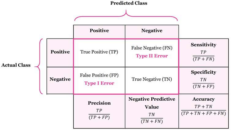
混淆矩阵
混淆矩阵 (Confusion Matrix )是一种用于评估分类模型性能的工具。它以矩阵形式展示了模型在不同类别上的预测结果与实际标签之间的对应关系。混淆矩阵的行表示实际类别,列表示预测类别。通过分析混淆矩阵,可以直观地了解模型在各个类别上的正确预测和错误预测情况,从而帮助识别模型的优势和不足,指导进一步的优化和改进。
真正例(True Positive, TP) :模型正确预测为正类的样本数量。假正例(False Positive, FP) :模型错误预测为正类的样本数量。真反例(True Negative, TN) :模型正确预测为负类的样本数量。假反例(False Negative, FN) :模型错误预测为负类的样本数量。
混淆矩阵的结构如下所示: