
Algo#2 Techniques Based on Recursion
Induction
Sort#2 Radix Sort
\begin{algorithm}
\caption{RADIXSORT}
	\begin{algorithmic}
		\Input A linked list of numbers $L = \{a_1 , a_2, . . . , a_n\}$ and $k$, the number of digits.
		\Output $L$ sorted in nondecreasing order.
		\For{$j \gets 1$ \To $k$}
	        \State Prepare 10 empty lists $L_0,L_1,\cdots,L_9$
	        \While{$L$ is \Not empty}
	            \State $a \gets$ next element in $L$.Delect $a$ from $L$.
	            \State $i \gets j$th digit in $a$.Append $a$ to list $L_i$.
            \EndWhile
            \State $L \gets L_0$
            \For{$i \gets 1$ \To 9}
	            \State $L \gets L,L_i$ \Comment{append list $L_i$ to $L$}
            \EndFor
        \EndFor
        \Return $L$
    \end{algorithmic}
\end{algorithm}
Below is the implementation of the pseudocode in Python:
1 | def RadixSort(arr, k): |
Integer Exponentiation
An efficient method can be deduced as follows. Let , and suppose we know how to compute . Then, we have two cases: If is even, then ; otherwise, .
\begin{algorithm}
\caption{EXPREC}
\begin{algorithmic}
\Input A real number $x$ and a nonnegative integet $n$.
\Output $x^n$
\State power($x$,$n$)
\Procedure{power}{$x,m$} \Comment{Compute $x^{m}$}
\If{$m$ = 0}
\State $y \gets 1$
\Else
	\State $y \gets \text{power}(x, \lfloor m/2 \rfloor)$
	\State $y \gets y^{2}$
	\If{$m$ is odd}
		\State $y \gets x \cdot y$
	\EndIf
\EndIf
\Return $y$
\EndProcedure
\end{algorithmic}
\end{algorithm}
\begin{algorithm}
\caption{EXP}
\begin{algorithmic}
\Input A real number $x$ and a nonnegative integet $n$.
\Output $x^n$
\STATE $y \gets 1$
\STATE Let $n$ be $d_k d_{k-1} \dots d_0$ in binary notation.
\FOR{$j \gets k$ \DOWNTO $0$}
    \STATE $y \gets y^{2}$
    \IF{$d_j = 1$}
        \STATE $y \gets x \cdot y$
    \ENDIF
\ENDFOR
\Return $y$
\end{algorithmic}
\end{algorithm}
Below is the implementation of these pseudocodes in Python:
1 | def exprec(x,n): |
Evaluating Polynomials (Horner’s Rule)
Suppose we have a sequence of real numbers and a real number , and we want to evaluate the polynomial
The straightforward approach would be to evaluate each term separately. This approach is very inefficient since it requires multiplications. A much faster method can be derived by induction as follows. We observe that
This evaluation scheme is known as Horner’s rule. Use of this scheme leads to the following more efficient method. Suppose we know how to evaluate
Then, using one more multiplication and one more addition, we have
This implies Algorithm HORNER.
\begin{algorithm}
\caption{HORNER}
\begin{algorithmic}
\Input A sequence of $n+1$ real numbers $a_0, a_1, \dots, a_n$ and a real number $x$.
\Output $P_n(x) = a_n x^n + a_{n-1} x^{n-1} + \dots + a_1 x + a_0$.
\State $p \gets a_n$
\For{$j \gets 1$ \to $n$}
    \State $p \gets x \cdot p + a_{n-j}$
\EndFor
\Return $p$
\end{algorithmic}
\end{algorithm}
Below is the implementation of the pseudocode in Python:
1 | def horner(A, x): |
or
1 | def horner(A, x): |
Generating Permutations
In this section, we study the problem of generating all permutations of the numbers .
The first algorithm
The algorithm uses a recursive backtracking approach to generate all permutations of an array by systematically swapping elements at different positions and exploring each arrangement through depth-first traversal. Note that interchanging back is necessary to restore the original state of the array for proper backtracking, ensuring all permutations are generated correctly without interference between recursive branches.
\begin{algorithm}
\caption{Permutations1}
\begin{algorithmic}
\Input A positive integer $n$.
\Output All permutations of the numbers $1,2,\cdots,n$.
\For{$j \gets 1$ \to $n$}
\State $P[j] \gets j$
\EndFor
\State \Call{perm1}{$1$}
\Procedure{perm1}{m}
\If{$m = n$}
\State \textbf{output} $P[1 \cdots n]$
\Else
\For{$j \gets m$ \to $n$}
\State interchange $P[j]$ and $P[m]$
\State \Call{perm1}{$m+1$}
\State interchange $P[j]$ and $P[m]$
\EndFor
\EndIf
\EndProcedure
\end{algorithmic}
\end{algorithm}
Below is the implementation of the pseudocode in Python:
1 | def perm1(m): |
Time complexity: .
The Second Algorithm
The algorithm uses backtracking to generate all permutations of the numbers 1 to n by recursively placing each number from n down to 1 in every available position.
\begin{algorithm}
\caption{Permutations2}
\begin{algorithmic}
\Input A positive integer $n$.
\Output All permutations of the numbers $1,2,\cdots,n$.
\For{$j \gets 1$ \to $n$}
\State $P[j] \gets 0$
\EndFor
\State \Call{perm2}{$n$}
\Procedure{perm2}{m}
\If{$m = 0$}
\State \textbf{output} $P[1 \cdots n]$
\Else
\For{$j \gets 1$ \to $n$}
\If{$P[j] = 0$}
\State $P[j] \gets m$
\State \Call{perm2}{$m-1$}
\State $P[j] \gets 0$
\EndIf
\EndFor
\EndIf
\EndProcedure
\end{algorithmic}
\end{algorithm}
Below is the implementation of the pseudocode in Python:
1 | n = 3 |
Finding the Majority Element
Let be a sequence of integers. An integer a in is called the majority if it appears more than times in .
Observation: If two different elements in the original sequence are removed, then the majority in the original sequence remains the majority in the new sequence.
This observation suggests the following procedure for finding an element that is a candidate for being the majority.
\begin{algorithm}
\caption{MAJORITY}
\begin{algorithmic}
\Input An array $A[1 \dots n]$ of $n$ elements.
\Output The majority element if it exists; otherwise none.
\State $c \gets$ \Call{candidate}{$1$}
\State $count \gets 0$
\For{$j \gets 1$ \to $n$}
\If{$A[j] = c$}
\State $count \gets count + 1$
\EndIf
\EndFor
\If{$count > \lfloor n/2 \rfloor$}
\Return $c$
\Else
\Return none
\EndIf

\Procedure{candidate}{$m$}
\State $j \gets m$
\State $c \gets A[m]$
\State $\textit{count} \gets 1$
\While{$j < n$ \and $\textit{count} > 0$}
    \State $j \gets j + 1$
    \If{$A[j] = c$}
        \State $\textit{count} \gets \textit{count} + 1$
    \Else
        \State $\textit{count} \gets \textit{count} - 1$
    \EndIf
\EndWhile
\If{$j = n$}
    \Return $c$
\Else
    \Return \Call{candidate}{$j + 1$}
\EndIf
\EndProcedure
\end{algorithmic}
\end{algorithm}
Below is the implementation of the pseudocode in Python:
1 | def candidate(m): |
Divide and Conquer
Binary Search
The binary search algorithm is a classic example of the divide-and-conquer paradigm. It works on a sorted array by repeatedly dividing the search interval in half. If the value of the search key is less than the item in the middle of the interval, narrow the interval to the lower half. Otherwise, narrow it to the upper half. Repeatedly check until the value is found or the interval is empty.
\begin{algorithm}
\caption{BINARYSEARCHREC}
\begin{algorithmic}
\Input An array $A[1..n]$ of $n$ elements sorted in nondecreasing order and an element $x$.
\Output $j$ if $x=A[j],1\leq j\leq n$, and $0$ otherwise.

\State binarysearch($1$, $n$)

\Procedure{binarysearch}{$low, high$}
    \If{$low > high$}
        \Return $0$
    \Else
        \State $mid \gets \lfloor (low + high) / 2 \rfloor$
        \If{$x = A[mid]$}
            \Return $mid$
        \ElsIf{$x < A[mid]$}
            \Return \Call{binarysearch}{$low$, $mid-1$}
        \Else
            \Return \Call{binarysearch}{$mid+1$, $high$}
        \EndIf
    \EndIf
\EndProcedure
\end{algorithmic}
\end{algorithm}
Below is the implementation of the pseudocode in Python:
1 | def binarysearch(low, high): |
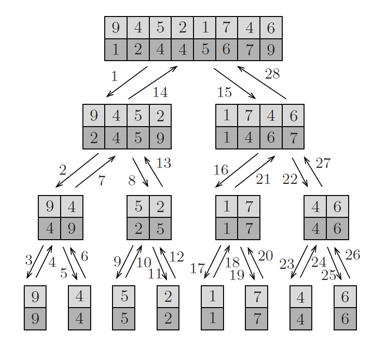
Sort#3 Mergesort
\begin{algorithm}
\caption{MERGESORT}
\begin{algorithmic}
\Input An array $A[1 \dots n]$ of $n$ elements.
\Output $A[1 \dots n]$ sorted in nondecreasing order.
\State \Call{mergesort}{$A$,$1$,$n$}
\Procedure{mergesort}{$A$,$low$,$high$}
\If{$low < high$}
\State $mid \gets \lfloor (low + high) / 2 \rfloor$
\State \Call{mergesort}{$A$,$low$,$mid$}
\State \Call{mergesort}{$A$,$mid+1$,$high$}
\State \Call{merge}{$A$,$low$,$mid$,$high$}
\EndIf
\EndProcedure
\end{algorithmic}
\end{algorithm}
The MERGE algorithm is discussed in Algo#1 Basic Concepts in Algorithmic Analysis | TheValuePoint’s Blog.
\begin{algorithm}
\caption{MERGE}
\begin{algorithmic}
\Input An array $A[1..m]$ of elements and three indices $p,q$, and $r$, with $1 \leq p \leq q < r \leq m$, such that both the subarrays $A[p..q]$ and $A[q+1..r]$ are sorted individually in nondecreasing order.
\Output $A[p..r]$ contains the result of merging the two subarrays $A[p..q]$ and $A[q+1..r]$.
\State \textbf{comment:} $B[p..r]$ is an auxiliary array.
\State $s \gets p$; $t \gets q+1$; $k \gets p$
\While{$s \leq q$ and $t \leq r$}
    \If{$A[s] \leq A[t]$}
        \State $B[k] \gets A[s]$
        \State $s \gets s + 1$
    \Else
        \State $B[k] \gets A[t]$
        \State $t \gets t + 1$
    \EndIf
    \State $k \gets k + 1$
\EndWhile
\If{$s = q + 1$}
    \State $B[k..r] \gets A[t..r]$
\Else
    \State $B[k..r] \gets A[s..q]$
\EndIf
\State $A[p..r] \gets B[p..r]$
\end{algorithmic}
\end{algorithm}
Below is the implementation of the MERGESORT pseudocode in Python:
1 | def merge(arr,p,q,r): |
Compared to the bottom-up sorting approach, merge sort is top-down.
\begin{algorithm}
\caption{BOTTOMUPSORT}
	\begin{algorithmic}
	\Input  An array $A[1..n]$ of $n$ elements.
	\Output $A[1..n]$ sorted in nondecreasing order.
	\State $t \gets 1$
	\While{$t < n$}
		\State $s \gets t; \quad t \gets 2s; \quad i \gets 0$
		\While{$i+t \leq n$}
			\State MERGE($A$, $i + 1$, $i + s$, $i + t$)
			\State $i \gets i+t$
	    \EndWhile
	    \If{$i+s < n$}
	    \State MERGE($A$, $i + 1$, $i + s$, n)
	    \EndIf
    \EndWhile
    \end{algorithmic}
\end{algorithm}
Selection: Finding the Median and the th Smallest Element
\begin{algorithm}
\caption{SELECT}
\begin{algorithmic}
\Input An array $A[1..n]$ of $n$ elements and an integer $k$, $1 \leq k \leq n$.
\Output The $k$th smallest element in $A$.
\Procedure{select}{$A,k$}
    \State $n \gets |A|$
    \If{$n < 44$}
        \State sort $A$
        \Return $A[k]$
    \EndIf
    \State $q \gets \lfloor n/5 \rfloor$
    \State Divide $A$ into $q$ groups of $5$ elements each. If $5$ does not divide $n$, discard the remaining elements.
    \State Sort each of the $q$ groups individually and extract its median. Let $M$ be the set of medians.
    \State $mm \gets \text{select}(M,\lceil q/2 \rceil)$ \Comment{median of medians}
    \State Partition $A$ into three arrays:
    \State $A_1 = \{ a \mid a < mm \}$
    \State $A_2 = \{ a \mid a = mm \}$
    \State $A_3 = \{ a \mid a > mm \}$
    \If{$|A_1| \geq k$}
        \Return $\text{select}(A_1,k)$
    \ElsIf{$|A_1| + |A_2| \geq k$}
        \Return $mm$
    \Else
        \Return $\text{select}(A_3,k - |A_1| - |A_2|)$
    \EndIf
\EndProcedure
\end{algorithmic}
\end{algorithm}
Below is the implementation of the pseudocode in Python:
1 | def select(A,low,high,k): |
Analysis of the selection algorithm
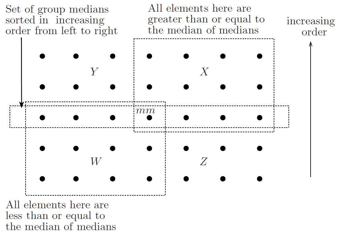
Assuming is the set of elements less than the median of medians and is the set of elements greater than the median of medians, we have
also
Now we are in a position to estimate , the running time of the algorithm. Steps 1 and 2 of procedure select in the algorithm cost time each. Step 3 costs time. Step 4 costs time, as sorting each group costs a constant amount of time. In fact, sorting each group costs no more than seven comparisons. The cost of Step 5 is . Step 6 takes time. By the above analysis, the cost of Step 7 is at most . Now we wish to express this ratio in terms of the floor function and get rid of the constant . For this purpose, let us assume that . Then, this inequality will be satisfied if , i.e., if . This is why we have set the threshold in the algorithm to . We conclude that the cost of this step is at most for . This analysis implies the following recurrence for the running time of Algorithm select.
for some constant that is sufficiently large. Since , it follows by Theorem 1.5, that the solution to this recurrence is . In fact, by Example 1.39,
Note that each ratio results in a different threshold. For instance, choosing results in a threshold of about . The following theorem summarizes the main result of this section.
The time complexity of Algorithm select is .
Sort#4 Quicksort
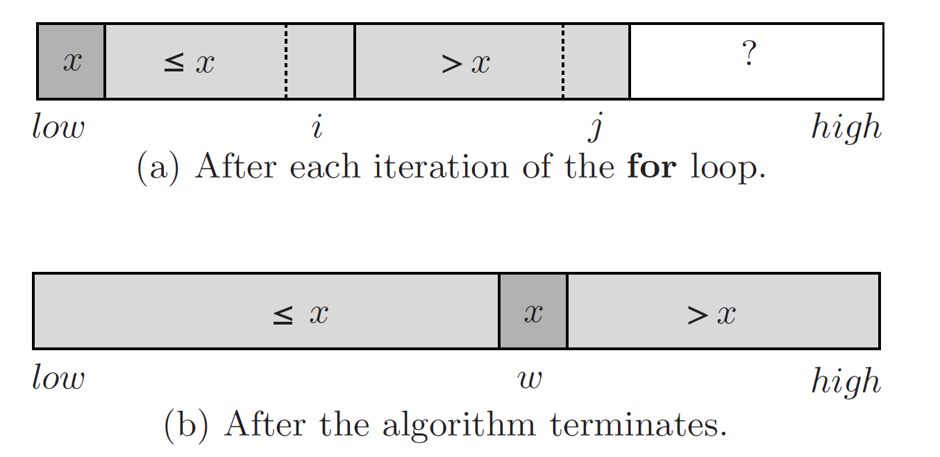
A partitioning algorithm
\begin{algorithm}
\caption{split}
\begin{algorithmic}
\Input An array of elements $A[low..high]$.
\Output (1) $A$ with its elements rearranged as described; (2) $w$, the new position of the splitting element $A[low]$.
    \State $i \gets low$
    \State $x \gets A[low]$
    \For{$j \gets low+1$ \textbf{to} $high$}
        \If{$A[j] \leq x$}
            \State $i \gets i + 1$
            \If{$i \neq j$}
                \State interchange $A[i]$ and $A[j]$
            \EndIf
        \EndIf
    \EndFor
    \State interchange $A[low]$ and $A[i]$
    \State $w \gets i$
    \Return $A$ and $w$
\end{algorithmic}
\end{algorithm}
The sorting algorithm
\begin{algorithm}
\caption{QUICKSORT}
\begin{algorithmic}
\Input An array $A[1..n]$ of $n$ elements.
\Output $A[1..n]$ sorted in nondecreasing order.
\State \Call{quicksort}{$A$,$1$,$n$}
\Procedure{quicksort}{$A$,$low$,$high$}
\If{$low < high$}
    \State \Call{split}{$A[low..high]$,$w$} \Comment{$w$ is the new position of $A[low]$}
    \State \Call{quicksort}{$A$,$low$,$w-1$}
    \State \Call{quicksort}{$A$,$w+1$,$high$}
\EndIf
\EndProcedure
\end{algorithmic}
\end{algorithm}
Below is the implementation of these pseudocodes in Python:
1 | def split(A, low, high): |
In the average case, the time complexity of quicksort is , while in the worst case, it can degrade to . Although no auxiliary storage is required by the algorithm to store the array elements, the space required by the algorithm is .
The Closest Pair Problem
\begin{algorithm}
\caption{CLOSESTPAIR}
\begin{algorithmic}
\Input A set $S$ of $n$ points in the plane.
\Output The minimum separation realized by two points in $S$.
\State Sort the points in $S$ in nondecreasing order of their $x$-coordinates.
\State $(\delta, Y) \gets $ \Call{cp}{1, n}
\Return $\delta$

\Procedure{cp}{$low, high$}
\If{$high - low + 1 \leq 3$}
    \State compute $\delta$ by a straightforward method.
    \State Let $Y$ contain the points in nondecreasing order of $y$-coordinates.
\Else
    \State $mid \gets \lfloor (low + high)/2 \rfloor$
    \State $x_0 \gets x(S[mid])$
    \State $(\delta_l, Y_l) \gets $ \Call{cp}{low, mid}
    \State $(\delta_r, Y_r) \gets $ \Call{cp}{mid + 1, high}
    \State $\delta \gets \min\{\delta_l, \delta_r\}$
    \State $Y \gets$ Merge $Y_l$ with $Y_r$ in nondecreasing order of $y$-coordinates.
    \State $k \gets 0$
    \For{$i \gets 1$ \To $|Y|$} \Comment{Extract $T$ from $Y$}
        \If{$|x(Y[i]) - x_0| \leq \delta$}
            \State $k \gets k + 1$
            \State $T[k] \gets Y[i]$
        \EndIf
    \EndFor \Comment{$k$ is the size of $T$}
    \State $\delta' \gets 2\delta$ \Comment{Initialize $\delta'$ to any number greater than $\delta$}
    \For{$i \gets 1$ \To $k - 1$} \Comment{Compute $\delta'$}
        \For{$j \gets i + 1$ \To $\min\{i + 7, k\}$}
            \If{$d(T[i], T[j]) < \delta'$}
                \State $\delta' \gets d(T[i], T[j])$
            \EndIf
        \EndFor
    \EndFor
    \State $\delta \gets \min\{\delta, \delta'\}$
\EndIf
\Return $(\delta, Y)$
\EndProcedure
\end{algorithmic}
\end{algorithm}
Below is the implementation of the pseudocode in Python:
1 | import math |
Dynamic Programming
The Longest Common Subsequence Problem
A simple problem that illustrates the principle of dynamic programming is the following. Given two strings and of lengths and , respectively, over an alphabet , determine the length of the longest subsequence that is common to both and . Here, a subsequence of is a string of the form , where each is between 1 and and . For example, if , and , then is a subsequence of length 3 of both and . However, it is not the longest common subsequence of and , since the string is also a common subsequence of length 4 of both and . Since these two strings do not have a common subsequence of length greater than 4, the length of the longest common subsequence of and is 4.
State Transition Equation:
\begin{algorithm}
\caption{LCS}
\begin{algorithmic}
\Input  Two strings $A$ and $B$ of lengths $n$ and $m$, respectively, over an alphabet $\Sigma$.
\Output The length of a longest common subsequence of $A$ and $B$.
\State $L[0, 0] \gets 0$
\For{$i \gets 1$ \To $n$}
    \State $L[i, 0] \gets 0$
\EndFor
\For{$j \gets 1$ \To $m$}
    \State $L[0, j] \gets 0$
\EndFor
\For{$i \gets 1$ \To $n$}
    \For{$j \gets 1$ \To $m$}
        \If{$a_i = b_j$}
            \State $L[i, j] \gets L[i - 1, j - 1] + 1$
        \Else
            \State $L[i, j] \gets \max(L[i - 1, j], L[i, j - 1])$
        \EndIf
    \EndFor
\EndFor
\Return $L[n, m]$
\End{Algorithmic}
\end{algorithm}
Below is the implementation of the pseudocode in Python:
1 | def LCS(A, B): |
Question Variant: The Longest Common Continuous Subsequence Problem
The longest common continuous subsequence problem, often referred to as the longest common substring problem, modifies the definition of a subsequence to require continuity. Given two strings and of lengths and , respectively, over an alphabet , the goal is to determine the length of the longest substring that appears consecutively in both and . Here, a substring of is a string of the form where . For example, using the same alphabet with and , the substring appears consecutively in both strings, as does the single character , but the common substring from the subsequence example is no longer valid because its characters are not contiguous in both strings. In this case, the longest common substring is with length 2. The problem illustrates a different dynamic programming approach, where the continuity constraint leads to a recurrence that resets the count when characters do not match, distinguishing it from the standard longest common subsequence problem.
State Transition Equation:
\begin{algorithm}
\caption{LCCS}
\begin{algorithmic}
\Input  Two strings $A$ and $B$ of lengths $n$ and $m$, respectively, over an alphabet $\Sigma$.
\Output The length of a longest common continuous subsequence of $A$ and $B$.
\State $L[0, 0] \gets 0$
\State $MaxLength \gets 0$
\For{$i \gets 1$ \To $n$}
    \State $L[i, 0] \gets 0$
\EndFor
\For{$j \gets 1$ \To $m$}
    \State $L[0, j] \gets 0$
\EndFor
\For{$i \gets 1$ \To $n$}
    \For{$j \gets 1$ \To $m$}
        \If{$a_{i-1} = b_{j-1}$}
            \State $L[i, j] \gets L[i - 1, j - 1] + 1$
            \State $MaxLength \gets \max(L[i, j],MaxLength)$
        \Else
            \State $L[i,j] \gets 0$
        \EndIf
    \EndFor
\EndFor
\Return $MaxLength$
\End{Algorithmic}
\end{algorithm}
Below is the implementation of the pseudocode in Python:
1 | def LCCS(A, B): |
The All-Pairs Shortest Path Problem: Floyd Algorithm
State Transition Equation:
Thus, in the th iteration, we compute using the formula
\begin{algorithm}
\caption{FLOYD}
\begin{algorithmic}
\Input An $n \times n$ matrix $l[1..n,1..n]$ such that $l[i,j]$ is the length of the edge $(i,j)$ in a directed graph $G = (\{1,2,\dots,n \},E)$.
\Output A matrix $D$ with $D[i,j] = $ the distance from $i$ to $j$.
\State $D \gets l$ \Comment{Copy the input matrix $l$ into $D$}
\For{$k \gets 1$ \To $n$}
    \For{$i \gets 1$ \To $n$}
        \For{$j \gets 1$ \To $n$}
            \State $D[i,j] \gets \min(D[i,j], D[i,k] + D[k,j])$
        \EndFor
    \EndFor
\EndFor
\end{algorithmic}
\end{algorithm}
Below is the implementation of the pseudocode in Python:
1 | def floyd(D): |
The Knapsack Problem
The knapsack problem can be defined as follows. Let be a set of items to be packed in a knapsack of size . For , let and be the size and value of the th item, respectively. Here and , are all positive integers. The objective is to fill the knapsack with some items from whose total size is at most and such that their total value is maximum. Assume without loss of generality that the size of each item does not exceed . More formally, given of items, we want to find a subset such that
is maximized subject to the constraint
This version of the knapsack problem is sometimes referred to in the literature as the 0/1 knapsack problem.
State Transition Equation:
\begin{algorithm}
\caption{KNAPSACK}
\begin{algorithmic}
\Input A set of items $U=\{u_{1},u_{2},\ldots,u_{n}\}$ with sizes $s_{1},s_{2},\ldots,s_{n}$ and values $v_{1},v_{2},\ldots,v_{n}$ and a knapsack capacity $C$.
\Output The maximum value of the function $\sum_{u_{i}\in S}v_{i}$ subject to $\sum_{u_{i}\in S}s_{i}\leq C$ for some subset of items $S\subseteq U$.

\For{$i\gets 0$ \To $n$}
    \State $V[i,0]\gets 0$
\EndFor
\For{$j\gets 0$ \To $C$}
    \State $V[0,j]\gets 0$
\EndFor
\For{$i\gets 1$ \To $n$}
    \For{$j\gets 1$ \To $C$}
        \State $V[i,j]\gets V[i-1,j]$
        \If{$s_{i}\leq j$}
            \State $V[i,j]\gets \max\{V[i,j], V[i-1,j-s_{i}]+v_{i}\}$
        \EndIf
    \EndFor
\EndFor
\Return $V[n,C]$
\end{algorithmic}
\end{algorithm}
Below is the implementation of the pseudocode in Python:
1 | def knapsack(S, V, C): |
Traveling Salesman Problem
Exercises 6.34 Give a dynamic programming algorithm for the traveling salesman problem: Given a set of cities with their intercity distances, find a tour of minimum length. Here, a tour is a cycle that visits each city exactly once. What is the time complexity of your algorithm? This problem can be solved using dynamic programming in time .