
Algo#3 First-Cut Techniques
The Greedy Approach
Dijkstra’s Algorithm
We define as the shortest known distance from the source vertex (vertex 1) to vertex . Initially, is set to the weight of the edge connecting vertex 1 to vertex if such an edge exists. If no such edge exists, is set to infinity (), indicating that vertex is not yet reachable from the source.
\begin{algorithm}
\caption{DIJKSTRA}
\begin{algorithmic}
\Input A weight directed graph $G = (V,E)$, where $V = \{ 1,2,\dots ,n \}$.
\Output The distance from vertex 1 to every other vertex in $G$.
\State $X = \{ 1 \}; \quad Y \gets V - \{ 1 \}; \quad \lambda [1] \gets 0$
\For{$y \gets 2$ \To $n$}
	\If{$y$ is adjacent to $1$ then $\lambda[y] \gets length[1,y]$}
    \Else
        \State $\lambda [y] \gets \infty$
    \EndIf
\EndFor
\For{$j \gets 1$ \To $n - 1$}
    \State Let $y \in Y$ be such that $\lambda[y]$ is minimum
    \State $X \gets X \cup \{y\}$ \Comment{add vertex $y$ to $X$}
    \State $Y \gets Y - \{y\}$ \Comment{delete vertex $y$ from $Y$}
    \For{each edge $(y, w)$}
        \If{$w \in Y$ and $\lambda[y] + length[y, w] < \lambda[w]$}
            \State $\lambda[w] \gets \lambda[y] + length[y, w]$
        \EndIf
    \EndFor
\EndFor
\end{algorithmic}
\end{algorithm}
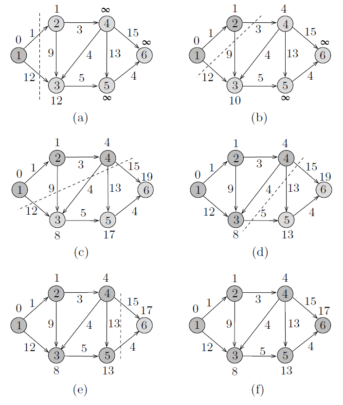
In the figure , those vertices to the left of the dashed line belong to , and the others belong to .
The time complexity of Dijkstra’s algorithm is .
Below is the implementation of the pseudocode in Python(Adjacency matrix):
1 | def Dijkstra(length): |
Minimum Cost Spanning Trees
Let be a connected undirected graph with weights on its edges. A spanning tree of is a subgraph of that is a tree. If is weighted and the sum of the weights of the edges in is minimum, then is called a minimum cost spanning tree or simply a minimum spanning tree.
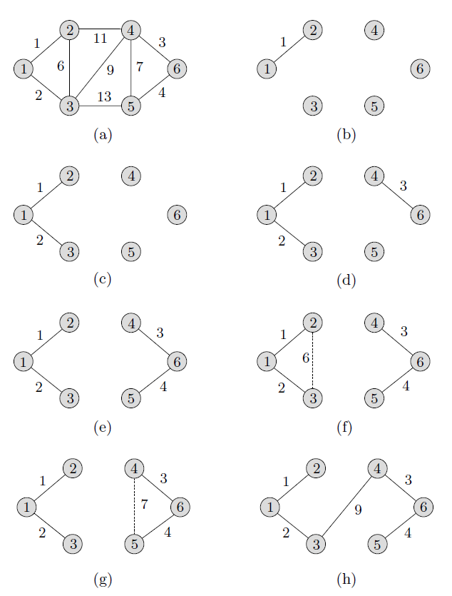
Kruskal’s Algorithm
\begin{algorithm}
\caption{KRUSKAL}
\begin{algorithmic}
\Input A weighted connected undirected graph $G = (V,E)$ with $n$ vertices.
\Output The set of edges $T$ of a minimum cost spanning tree for $G$.
\State Sort the edges in $E$ by nondecreasing weight.
\For{each vertex $v \in V$}
    \State \Call{makeset}{$\{v\}$}
\EndFor
\State $T \gets \{\}$
\While{$|T| < n - 1$}
    \State Let $(x, y)$ be the next edge in $E$.
    \If{\Call{find}{$x$} $\neq$ \Call{find}{$y$}}
        \State \Call{add}{$x, y$} to $T$
        \State \Call{union}{$x, y$}
    \EndIf
\EndWhile
\end{algorithmic}
\end{algorithm}
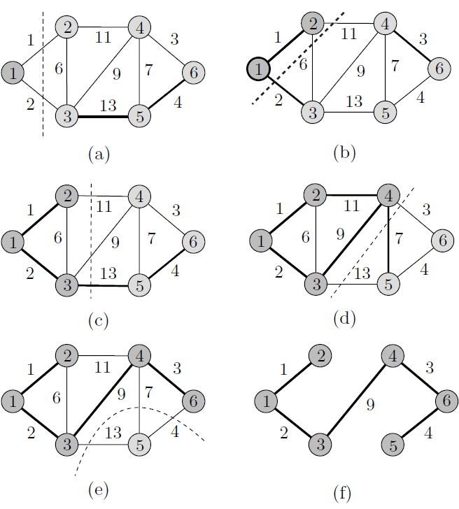
Prim’s Algorithm
\begin{algorithm}
\caption{PRIM}
\begin{algorithmic}
\Input A weighted connected undirected graph $G = (V, E)$, where $V = \{1, 2, \dots, n\}$.
\Output The set of edges $T$ of a minimum cost spanning tree for $G$.
\State $T \gets \{\}; \quad X \gets \{1\}; \quad Y \gets V - \{1\}$
\For{$y \gets 2$ \To $n$}
    \If{$y$ is adjacent to $1$}
        \State $N[y] \gets 1$
        \State $C[y] \gets c[1, y]$
    \Else
        \State $C[y] \gets \infty$
    \EndIf
\EndFor
\For{$j \gets 1$ \To $n - 1$} \Comment{find $n - 1$ edges}
    \State Let $y \in Y$ be such that $C[y]$ is minimum
    \State $T \gets T \cup \{(y, N[y])\}$ \Comment{add edge $(y, N[y])$ to $T$}
    \State $X \gets X \cup \{y\}$ \Comment{add vertex $y$ to $X$}
    \State $Y \gets Y - \{y\}$ \Comment{delete vertex $y$ from $Y$}
    \For{each vertex $w \in Y$ that is adjacent to $y$}
        \If{$c[y, w] < C[w]$}
            \State $N[w] \gets y$
            \State $C[w] \gets c[y, w]$
        \EndIf
    \EndFor
\EndFor
\end{algorithmic}
\end{algorithm}
Huffman tree
\begin{algorithm}
\caption{HUFFMAN}
\begin{algorithmic}
\Input A set $C = \{c_1, c_2, \dots, c_n\}$ of $n$ characters and their frequencies $\{f(c_1), f(c_2), \dots, f(c_n)\}$.
\Output A Huffman tree $(V, T)$ for $C$.
\State Insert all characters into a min-heap $H$ according to their frequencies.
\State $V \gets C; \quad T \gets \{\}$
\For{$j \gets 1$ \To $n - 1$}
    \State $c \gets $\Call{deletemin}{H}
    \State $c' \gets $\Call{deletemin}{H}
    \State $f(v) \gets f(c) + f(c')$ \Comment{$v$ is a new node}
    \State \Call{insert}{$H, v$}
    \State $V \gets V \cup \{v\}$ \Comment{Add $v$ to $V$}
    \State $T \gets T \cup \{(v, c), (v, c')\}$ \Comment{Make $c$ and $c'$ children of $v$ in $T$}
\EndFor
\end{algorithmic}
\end{algorithm}
The time complexity of the algorithm is .
Graph Traversal
Depth-First Search
\begin{algorithm}
\caption{DFS}
\begin{algorithmic}
\Input A (directed or undirected) graph $G = (V, E)$.
\Output Preordering and postordering of the vertices in the corresponding depth-first search tree.
\State $predfn \gets 0; \quad postdfn \gets 0$
\For{each vertex $v \in V$}
    \State mark $v$ unvisited
\EndFor
\For{each vertex $v \in V$}
    \If{$v$ is marked unvisited}
        \State \Call{dfs}{$v$}
    \EndIf
\EndFor
\Procedure{dfs}{$v$}
    \State mark $v$ visited
    \State $predfn \gets predfn + 1$
    \For{each edge $(v, w) \in E$}
        \If{$w$ is marked unvisited}
            \State \Call{dfs}{$w$}
        \EndIf
    \EndFor
    \State $postdfn \gets postdfn + 1$
\EndProcedure
\end{algorithmic}
\end{algorithm}
Breadth-First Search
\begin{algorithm}
\caption{BFS}
\begin{algorithmic}
\Input A (directed or undirected) graph $G = (V, E)$.
\Output Numbering of the vertices in breadth-first search order.
\State $bfn \gets 0$
\For{each vertex $v \in V$}
    \State mark $v$ unvisited
\EndFor
\For{each vertex $v \in V$}
    \If{$v$ is marked unvisited}
        \State \Call{bfs}{$v$}
    \EndIf
\EndFor
\Procedure{bfs}{$v$}
    \State $Q \gets \{v\}$
    \State mark $v$ visited
    \While{$Q \neq \{\}$}
        \State $v \gets$ \Call{Pop}{$Q$}
        \State $bfn \gets bfn + 1$
        \For{each edge $(v, w) \in E$}
            \If{$w$ is marked unvisited}
                \State \Call{Push}{$w, Q$}
                \State mark $w$ visited
            \EndIf
        \EndFor
    \EndWhile
\EndProcedure
\end{algorithmic}
\end{algorithm}
Finding Articulation Points in a Graph
A vertex in an undirected graph with more than two vertices is called an articulation point if there exist two vertices and different from such that any path between and must pass through . Thus, if is connected, the removal of and its incident edges will result in a disconnected subgraph of . A graph is called biconnected if it is connected and has no articulation points.
To find the set of articulation points, we perform a depth-first search traversal on . During the traversal, we maintain two labels with each vertex : and . is simply predfn in the depth-first search algorithm, which is incremented at each call to the depth-first search procedure. is initialized to , but may change later on during the traversal. For each vertex visited, we let be the minimum of the following:
- .
- for each vertex such that is a back edge.
- for each edge in the depth-first search tree.
The articulation points are determined as follows: - The root is an articulation point if and only if it has two or more children in the depth-first search tree.
- A vertex other than the root is an articulation point if and only if has a child with .
The formal algorithm for finding the articulation points is given as AlgorithmARTICPOINTS.
\begin{algorithm}
\caption{ARTICPOINTS}
\begin{algorithmic}
\Input A connected undirected graph $G = (V, E)$.
\Output Array $A[1..count]$ containing the articulation points of $G$, if any.
\State Let $s$ be the start vertex.
\For{each vertex $v \in V$}
    \State mark $v$ unvisited
\EndFor
\State $predfn \gets 0; \quad count \gets 0; \quad rootdegree \gets 0$
\State \Call{dfs}{$s$}
\Procedure{dfs}{$v$}
    \State mark $v$ visited; $artpoint \gets \textbf{false}$; $predfn \gets predfn + 1$
    \State $\alpha[v] \gets predfn; \quad \beta[v] \gets predfn$ \Comment{Initialize $\alpha[v]$ and $\beta[v]$}
    \For{each edge $(v, w) \in E$}
        \If{$(v, w)$ is a tree edge}
            \State \Call{dfs}{$w$}
            \If{$v = s$}
                \State $rootdegree \gets rootdegree + 1$
                \If{$rootdegree = 2$}
                    \State $artpoint \gets \textbf{true}$
                \EndIf
            \Else
                \State $\beta[v] \gets \min\{\beta[v], \beta[w]\}$
                \If{$\beta[w] \geq \alpha[v]$}
                    \State $artpoint \gets \textbf{true}$
                \EndIf
            \EndIf
        \ElsIf{$(v, w)$ is a back edge}
            \State $\beta[v] \gets \min\{\beta[v], \alpha[w]\}$
        \Else
            \State \textbf{do nothing} \Comment{$w$ is the parent of $v$}
        \EndIf
    \EndFor
    \If{$artpoint$}
        \State $count \gets count + 1$
        \State $A[count] \gets v$
    \EndIf
\EndProcedure
\end{algorithmic}
\end{algorithm}
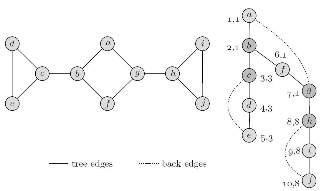
We illustrate the action of Algorithm ARTICPOINTS by finding the articulation points of the graph shown in the figure. See the figure. Each vertex in the depth-first search tree is labeled with and . The depth-first search starts at vertex and proceeds to vertex . A back edge is discovered, and hence is assigned the value . Now, when the search backs up to vertex , is assigned . Similarly, when the search backs up to vertex , its label is assigned the value . Now, since , vertex is marked as an articulation point. When the search backs up to , it is also found that , and hence is also marked as an articulation point. At vertex , the search branches to a new vertex and proceeds, as illustrated in the figure, until it reaches vertex . The back edge is detected and hence is set to . Now, as described before, the search backs up to and then and sets and to . Again, since , vertex is marked as an articulation point. For the same reason, vertex is marked as an articulation point. At vertex , the back edge is detected, and hence is set to . Finally, and then are set to and the search terminates at the start vertex. The root is not an articulation point since it has only one child in the depth-first search tree.
Below is the implementation of the pseudocode in Python(Adjacency list):
1 | graph = { |